Ozkan pTO Method: Deng Entropy-Based Taxonomic Diversity
Source:vignettes/ozkan-pto.Rmd
ozkan-pto.RmdWhat Is the Ozkan pTO Method?
Ozkan (2018) introduced a novel approach to measuring taxonomic diversity using Deng entropy — a generalization of Shannon entropy rooted in Dempster-Shafer evidence theory (Dempster, 1967; Shafer, 1976). Ozkan & Mert (2022) extended this with reinforced estimators that use stochastic resampling (Run 2) and sensitivity analysis (Run 3) to refine the indices.
The key idea: at each level of the taxonomic hierarchy (genus, family, order, etc.), Deng entropy measures how evenly species are distributed across groups. The product of these level-wise entropies gives a single number that captures the entire hierarchical diversity of a community.
This approach produces 8 complementary indices through a three-stage pipeline, each answering a slightly different question about the community.
library(taxdiv)

community <- c(
  Quercus_coccifera    = 9,
  Quercus_infectoria   = 7,
  Pinus_brutia         = 9,
  Pinus_nigra          = 5,
  Juniperus_excelsa    = 4,
  Juniperus_oxycedrus  = 3,
  Arbutus_andrachne    = 6,
  Styrax_officinalis   = 2,
  Cercis_siliquastrum  = 1,
  Olea_europaea        = 5
)

tax_tree <- build_tax_tree(
  species = names(community),
  Genus   = c("Quercus", "Quercus", "Pinus", "Pinus",
              "Juniperus", "Juniperus", "Arbutus", "Styrax",
              "Cercis", "Olea"),
  Family  = c("Fagaceae", "Fagaceae", "Pinaceae", "Pinaceae",
              "Cupressaceae", "Cupressaceae", "Ericaceae", "Styracaceae",
              "Fabaceae", "Oleaceae"),
  Order   = c("Fagales", "Fagales", "Pinales", "Pinales",
              "Pinales", "Pinales", "Ericales", "Ericales",
              "Fabales", "Lamiales")
)
From Shannon to Deng: Why a New Entropy?
Shannon entropy treats each species as an independent event with probability . But in a taxonomic hierarchy, species are grouped — two oak species share more information than an oak and a pine. Shannon cannot capture this grouping.
Deng entropy solves this through the concept of focal elements from evidence theory. At each taxonomic level, a group (e.g., “Family Fagaceae”) acts as a focal element with a mass proportional to the species it contains. The entropy accounts for both the mass distribution and the size of each focal element (how many species it contains):
where is the mass of focal element and is the number of species it contains.
The term accounts for all possible non-empty subsets of species within the group. A genus with 3 species has possible subcombinations, giving it more “evidential weight” than a single-species genus.
Deng Entropy at Each Taxonomic Level
result <- ozkan_pto(community, tax_tree)

cat("Deng entropy by taxonomic level:\n\n")
#> Deng entropy by taxonomic level:
for (i in seq_along(result$Ed_levels)) {
  level <- names(result$Ed_levels)[i]
  value <- result$Ed_levels[i]
  cat(sprintf("  %-10s Ed = %.4f\n", level, value))
}
#>   Species    Ed = 2.3026
#>   Genus      Ed = 2.5459
#>   Family     Ed = 2.5459
#>   Order      Ed = 2.9935
How to interpret:
- Species level: Equals Shannon entropy when all species are equally weighted (special case where each focal element has size 1)
- Genus level: High when species are spread across many genera. Low when most species share one genus.
- Family level: High when genera span many families. Low when the community is taxonomically narrow at the family level.
- Order level: Similar pattern at the highest taxonomic rank.
A level with Deng entropy = 0 means all species belong to a single group at that level — it contributes no taxonomic information.
The 8 Indices Explained
The Ozkan method produces 8 values organized in a 2 x 2 x 2 structure:
Weighted vs Unweighted
- Unweighted (u): Each taxonomic level contributes equally to the product
- Weighted: Higher taxonomic levels receive more weight (because resolving diversity at the order level is “more valuable” than at the genus level)
With vs Without Species-Level Shannon
- pTO: Product of Deng entropies across taxonomic levels only (genus, family, order) — pure taxonomic structure
- pTO+: Same product, but also includes the species-level Shannon entropy — captures both abundance evenness and taxonomic structure
All Levels vs Max-Informative Levels
- Standard: Uses all taxonomic levels
- Max variants: Uses only levels where Deng entropy > 0 (drops uninformative levels)
cat("=== All 8 Ozkan pTO indices ===\n\n")
#> === All 8 Ozkan pTO indices ===
cat("Standard (all levels):\n")
#> Standard (all levels):
cat("  uTO      =", round(result$uTO, 4), "  (unweighted diversity)\n")
#>   uTO      = 7.7613   (unweighted diversity)
cat("  TO       =", round(result$TO, 4), "  (weighted diversity)\n")
#>   TO       = 10.9393   (weighted diversity)
cat("  uTO+     =", round(result$uTO_plus, 4), "  (unweighted distance)\n")
#>   uTO+     = 8.5502   (unweighted distance)
cat("  TO+      =", round(result$TO_plus, 4), "  (weighted distance)\n\n")
#>   TO+      = 11.7283   (weighted distance)

cat("Max-informative levels:\n")
#> Max-informative levels:
cat("  uTO_max  =", round(result$uTO_max, 4), "  (unweighted, informative only)\n")
#>   uTO_max  = 7.7613   (unweighted, informative only)
cat("  TO_max   =", round(result$TO_max, 4), "  (weighted, informative only)\n")
#>   TO_max   = 10.9393   (weighted, informative only)
cat("  uTO+_max =", round(result$uTO_plus_max, 4), "  (unweighted distance, informative only)\n")
#>   uTO+_max = 8.5502   (unweighted distance, informative only)
cat("  TO+_max  =", round(result$TO_plus_max, 4), "  (weighted distance, informative only)\n")
#> TO+_max = 11.7283 (weighted distance, informative only)The Three-Run Pipeline
Run 2: Stochastic Resampling (Slicing)
Species are removed one at a time, starting with the least abundant. After each removal, all indices are recalculated. This “slicing” procedure reveals two things:
- The maximum diversity achievable from the community’s species pool
- Each species’ contribution to overall diversity
run2 <- ozkan_pto_resample(community, tax_tree, n_iter = 101, seed = 42)

cat("Run 1 (deterministic):  uTO+ =", round(run2$uTO_plus_det, 4), "\n")
#> Run 1 (deterministic):  uTO+ = 8.5502
cat("Run 2 (stochastic max): uTO+ =", round(run2$uTO_plus_max, 4), "\n")
#> Run 2 (stochastic max): uTO+ = 8.5502
Why does maximum > deterministic? Because some species may be taxonomically redundant. If two species from the same genus are present, removing one can increase the ratio of between-group to within-group diversity. The species whose removal increases diversity is called an “unhappy” species — it is taxonomically redundant in the community.
Visualizing Run 2
plot_iteration(run2, component = "TO_plus",
               title = "Run 2: TO+ Across Iterations")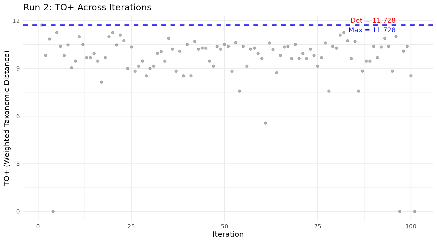
How to read:
- Grey dots: pTO value for each random species subset
- Red line: Deterministic value (Run 1 — all species included)
- Blue line: Maximum value found (Run 2 result)
Points above the red line represent subcommunities more diverse than the full community — evidence that some species are taxonomically redundant.
Run 3: Max-Informative Level Variants
Some taxonomic levels carry no information. If all species belong to the same order, Deng entropy at the order level is zero — including it in the product just drags the value down without adding insight.
Run 3 repeats the calculation using only levels where Deng entropy > 0:
run3 <- ozkan_pto_sensitivity(community, tax_tree, run2, seed = 123)

cat("All levels:       TO+ =", round(run3$TO_plus_max, 4), "\n")
#> All levels:       TO+ = 11.7283
cat("Informative only: TO+ =", round(result$TO_plus_max, 4), "\n")
#> Informative only: TO+ = 11.7283
Full Pipeline in One Call
full <- ozkan_pto_full(community, tax_tree, n_iter = 101, seed = 42)

cat("Complete pipeline summary:\n\n")
#> Complete pipeline summary:
cat("         uTO+      TO+       uTO       TO\n")
#>          uTO+      TO+       uTO       TO
cat("Run 1:", sprintf("%9.4f %9.4f %9.4f %9.4f",
    full$run1$uTO_plus, full$run1$TO_plus,
    full$run1$uTO, full$run1$TO), "\n")
#> Run 1:    8.5502   11.7283    7.7613   10.9393
cat("Run 2:", sprintf("%9.4f %9.4f %9.4f %9.4f",
    full$run2$uTO_plus_max, full$run2$TO_plus_max,
    full$run2$uTO_max, full$run2$TO_max), "\n")
#> Run 2:    8.5502   11.7283    7.7613   10.9393
cat("Run 3:", sprintf("%9.4f %9.4f %9.4f %9.4f",
    full$run3$uTO_plus_max, full$run3$TO_plus_max,
    full$run3$uTO_max, full$run3$TO_max), "\n")
#> Run 3:    8.5502   11.7283    7.7613   10.9393
Jackknife Leave-One-Out Analysis
The jackknife procedure removes each species one at a time and recalculates all indices. This directly measures each species’ contribution:
jk <- ozkan_pto_jackknife(community, tax_tree)

cat("Jackknife results (TO+ when each species is removed):\n\n")
#> Jackknife results (TO+ when each species is removed):
jk_df <- jk$jackknife_results
for (i in seq_len(nrow(jk_df))) {
  direction <- ifelse(jk_df$TO_plus[i] > result$TO_plus, "UNHAPPY", "happy")
  cat(sprintf("  Remove %-25s -> TO+ = %.4f  [%s]\n",
              jk_df$species[i], jk_df$TO_plus[i], direction))
}
#>   Remove Quercus_coccifera         -> TO+ = 11.4820  [happy]
#>   Remove Quercus_infectoria        -> TO+ = 11.4820  [happy]
#>   Remove Pinus_brutia              -> TO+ = 11.6616  [happy]
#>   Remove Pinus_nigra               -> TO+ = 11.6616  [happy]
#>   Remove Juniperus_excelsa         -> TO+ = 11.6616  [happy]
#>   Remove Juniperus_oxycedrus       -> TO+ = 11.6616  [happy]
#>   Remove Arbutus_andrachne         -> TO+ = 11.3238  [happy]
#>   Remove Styrax_officinalis        -> TO+ = 11.3238  [happy]
#>   Remove Cercis_siliquastrum       -> TO+ = 11.2505  [happy]
#>   Remove Olea_europaea             -> TO+ = 11.2505  [happy]

cat("\nHappy species:", jk$n_happy, "\n")
#>
#> Happy species: 10
cat("Unhappy species:", jk$n_unhappy, "\n")
#> Unhappy species: 0- happy species: Removing them decreases diversity (they contribute positively to taxonomic structure)
- UNHAPPY species: Removing them increases diversity (they are taxonomically redundant)
Comparing Communities
degraded <- c(
  Quercus_coccifera   = 9,
  Pinus_brutia        = 8,
  Juniperus_oxycedrus = 5
)

communities <- list(
  "Intact (10 spp)"  = community,
  "Degraded (3 spp)" = degraded
)

plot_radar(communities, tax_tree,
           title = "Intact vs Degraded Forest")
#> Warning: Removed 2 rows containing missing values or values outside the scale range
#> (`geom_point()`).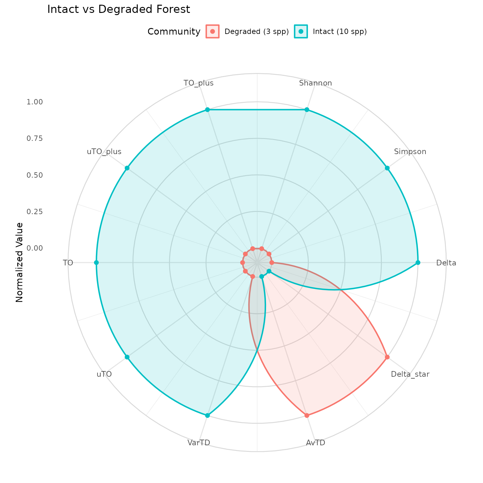
The radar chart reveals which diversity dimensions are most affected by degradation. If abundance-weighted indices (Shannon, Simpson, TO+) drop more than presence/absence indices (AvTD, uTO+), the community has lost evenness. If both drop equally, the community has lost taxonomic breadth.
References
- Ozkan, K. (2018). A new proposed measure for estimating taxonomic diversity. Turkish Journal of Forestry, 19(4), 336-346.
- Ozkan, K. & Mert, A. (2022). Comparisons of Deng entropy-based taxonomic diversity measures with the other diversity measures and introduction to the new proposed (reinforced) estimators. FORESTIST, 72(2). doi: 10.5152/forestist.2021.21025
- Deng, Y. (2016). Deng entropy. Chaos, Solitons & Fractals, 91, 549-553.
- Dempster, A.P. (1967). Upper and lower probabilities induced by a multivalued mapping. The Annals of Mathematical Statistics, 38(2), 325-339.
- Shafer, G. (1976). A Mathematical Theory of Evidence. Princeton University Press, Princeton, NJ.