Funnel Plot for AvTD/VarTD

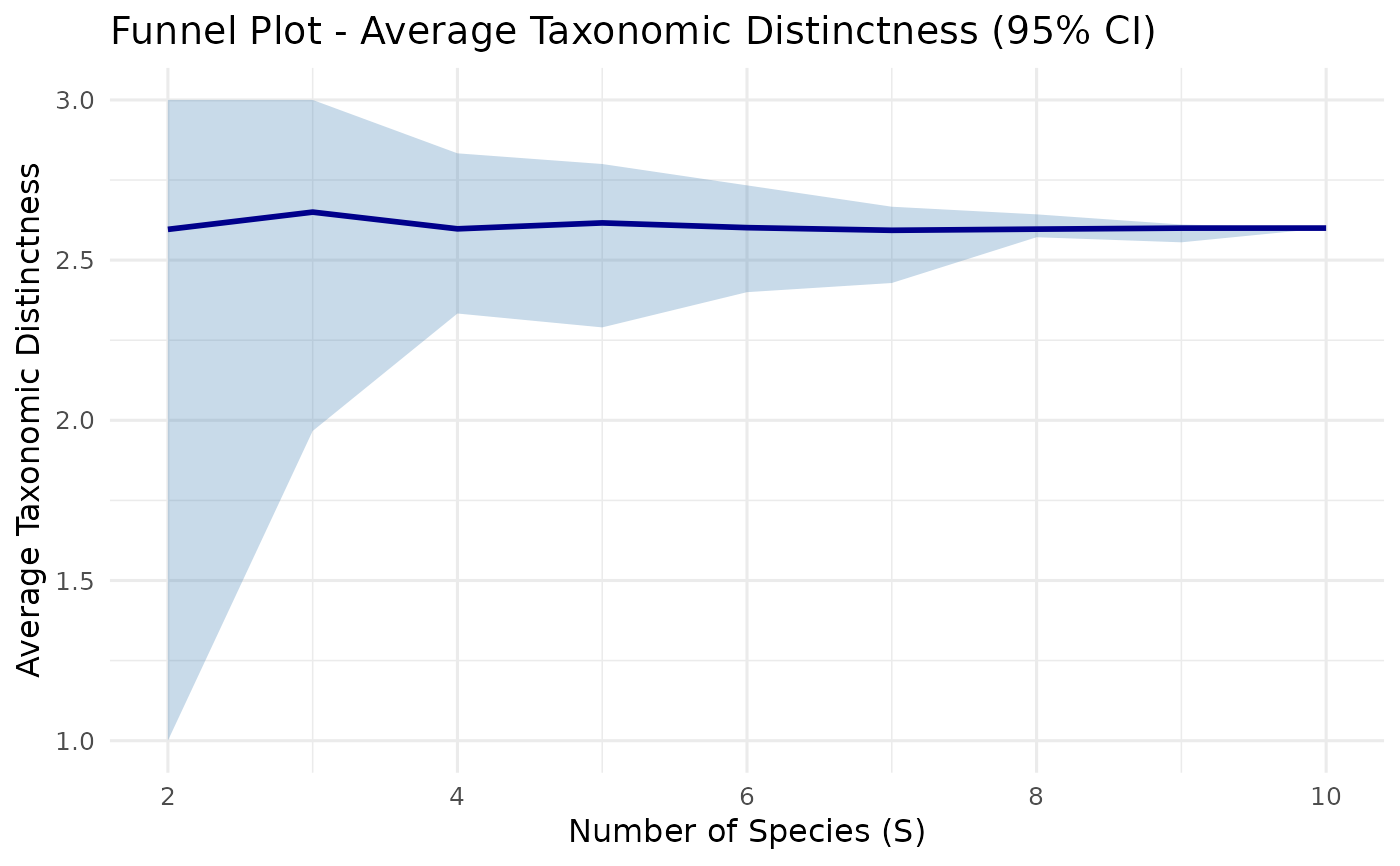
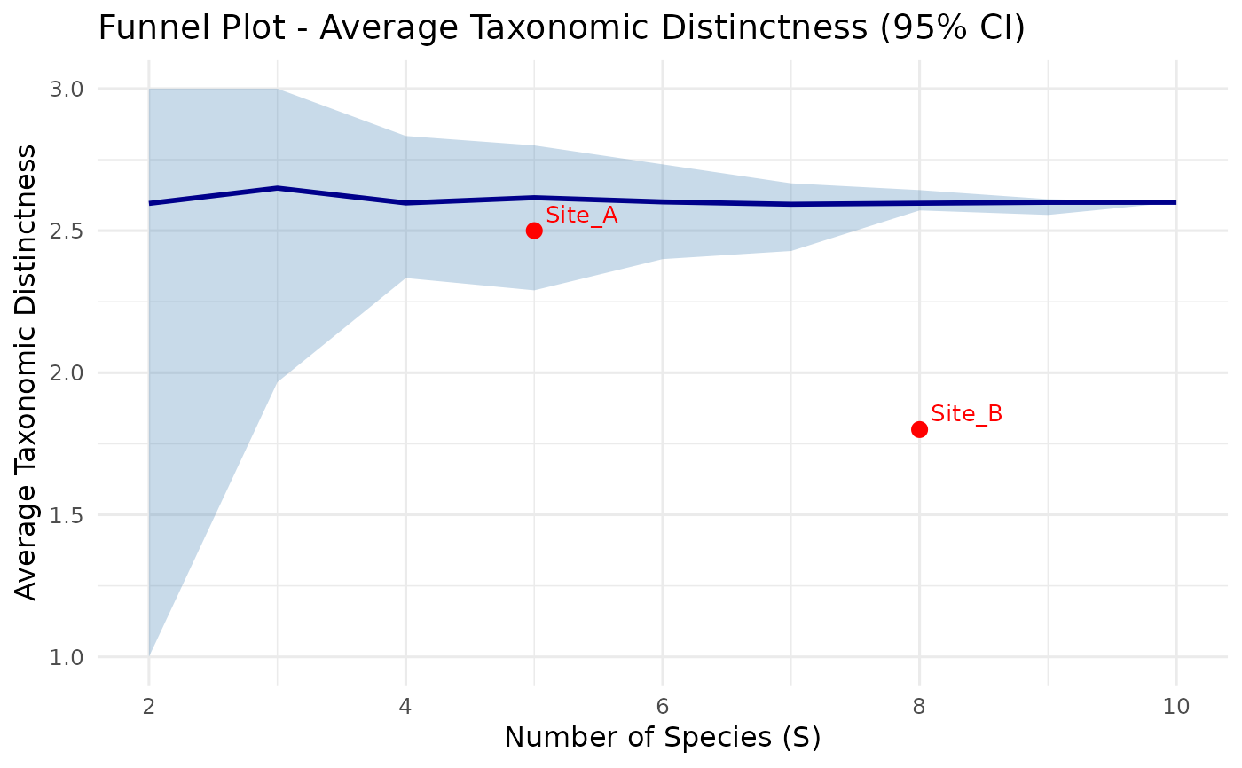
Produces a Clarke & Warwick style funnel plot showing expected confidence limits for Average Taxonomic Distinctness (AvTD) and/or Variation in Taxonomic Distinctness (VarTD) as a function of species richness. Observed site values can be overlaid to assess whether they fall within or outside the expected range.

Usage

plot_funnel(
  sim_result,
  observed = NULL,
  index = c("avtd", "vartd"),
  title = NULL,
  point_labels = TRUE,
  mean_color = "darkblue",
  ci_color = "steelblue"
)

Arguments

sim_result

A td_simulation object returned by simulate_td().

observed

Optional data frame with columns site (character), s (integer, species richness), and value (numeric, observed AvTD or VarTD). Points are plotted on the funnel.

index

Which index to plot when sim_result contains both: "avtd" (default) or "vartd".

title

Optional plot title. If NULL, generated automatically.

point_labels

Logical; if TRUE (default), label observed points with site names.

mean_color

Color of the mean line (default: "darkblue").

ci_color

Fill color of the confidence band (default: "steelblue").

Value

A ggplot object.

Details

The funnel shape arises because small samples (low S) have greater random variation in AvTD/VarTD, producing wider confidence bands. As S approaches the full species pool, the band narrows.

Observed points falling below the lower confidence limit suggest the community has lower taxonomic breadth than expected by chance, potentially indicating environmental stress or biotic homogenisation.

Requires the ggplot2 package.

References

Clarke, K.R. & Warwick, R.M. (1998). A taxonomic distinctness index and its statistical properties. Journal of Applied Ecology, 35, 523-531.

See also

simulate_td() for generating the simulation, avtd() and vartd() for the underlying calculations.

Examples

# \donttest{
tax <- data.frame(
  Species = paste0("sp", 1:10),
  Genus   = rep(c("G1", "G2", "G3", "G4", "G5"), each = 2),
  Family  = rep(c("F1", "F1", "F2", "F2", "F3"), each = 2),
  Order   = rep(c("O1", "O1", "O2", "O2", "O2"), each = 2),
  stringsAsFactors = FALSE
)
sim <- simulate_td(tax, n_sim = 99, seed = 42)

# Basic funnel plot
plot_funnel(sim)


# With observed sites
obs <- data.frame(
  site  = c("Site_A", "Site_B"),
  s     = c(5, 8),
  value = c(2.5, 1.8)
)
plot_funnel(sim, observed = obs)

# }